1 Concepts and measures

Learning objectives

• Learn what demography is and why it’s important
• Know how to specify a population in demographic terms
• Apply the balancing equation and its main components to track change in population size over time
• Learn what person-periods are and how to approximate them
• Use occurrences, person-periods, and observations to construct demographic rates and probabilities
• Understand the differences between rates and probabilities
• Learn the relationships and differences between crude, instantaneous, and mean annualized growth rates
• Learn the differences between a period and a cohort, and their relation to rates and probabilities

1.1 What is demography and why is it important?

Definitions of demography

• “…the scientific study of human populations primarily with respect to their size, their structure and their development; it takes into account the quantitative aspects of their general characteristics.⁶
• The study of human populations in relation to the changes brought about by the interplay of births, deaths, and migration.⁷
• “…the study of of human populations – their size, composition and distribution across space – and the process through which populations change.⁸

Emphasis added.

Discussion questions

What are the “processes” that the Stockholm University Demographic Unit’s definition drives at? Tap for answer

• Birth: Entering the population from the womb
• Death: Exiting the population because we’re all mortal
• Migration: Physically moving in our out of the population’s location

What are three basic dimensions along which these changes occur? Tap for answer

• Time: For example, you can track the number of deaths from year to year
• Space: You can track how a population moves its location over time, or how individuals move into our out of a local population over time.
• Structure: You can disaggregate a population into subpopulations. For example, by age, by race or ethnicity, by religion, by gender. This structure may change over time.

Okay so what’s a “population” then?

For statistians: A collection of items

For demographers:

1. A collection of persons…
2. who meet certain criteria
3. alive at a specified point in time…
   
   

Anything odd about point 1 above? Tap for answer

Non-human biologists do demography, too.

• Dr. Hal Caswell, Professor of Mathematical Demography at University of Amsterdam: https://www.uva.nl/en/profile/c/a/h.caswell/h.caswell.html
• Wrote influential book on matrix population models (aka… demography)

“My research focuses on population models, usually based on matrices, for plants, [non-human] animals, and humans. I am interested in stochastic processes in demography…”

– Hal Caswell (my emphasis)

Let’s think of some examples. Tap for answer

• Collection: People…
• Criteria: living in King County, Washington…
• Specified point in time: on April 1, 2019

2.3 M people⁹

Also for demographers:

Population as an enduring collection of individuals

By “enduring,” PHG mean those characteristics of a population that don’t change.

Extending our Seattle metro example to “enduring” collections Tap for answer

Now we can see how the population changes, in this case over time…

King County population grew by 28% over 14 years.

And here is a more interactive example from Italy made by Eddie Hunsinger: https://shiny.demog.berkeley.edu/eddieh/lx_ndx_Italy/, which we’ll return to in week 3

1.2 The balancing equation of population change

• Consider an observation period of length \(T\)
• For now, arbitrarily set the period’s starting point at time \(t = 0\)

\(\begin{align} N(T) &= \textsf{ (Ending population size at time } T \textsf{)} \\ &+ N(0) \textsf{ (Starting population size at time } 0 \textsf{)} \\ &+ B[0,T] \textsf{ (Number of births from start to end)} \\ &- D[0,T] \textsf{ (Number of deaths from start to end)} \\ &+ I[0,T] \textsf{ (Number in-migrations from start to end)} \\ &- O[0,T] \textsf{ (Number out-migrations from start to end)} \\ \end{align}\)

Organized by ways to enter vs. exit a population… Tap for answer

\(\begin{align} N(T) &= N(0) \\ &+ B[0,T] + I[0,T] \textsf{ (Ways to enter)} \\ &- D[0,T] - O[0,T] \textsf{ (Ways to exit)} \end{align}\)

Organized by natural increase vs. net migration… Tap for answer

\(\begin{align} NI[0,T] &= B[0,T] - D[0,T] \textsf{ (Natural increase)} \\ NM[0,T] &= I[0,T] - O[0,T] \textsf{ (Net migration)} \end{align}\)

And putting it all together… Tap for answer

\(N(T) = N[0] + NI[0,T] + NM[0,T]\)

Balancing equation as flows and stocks

• Boxes represent states that individuals in a population can be in
• Arrows represent a flow of individuals from one state to another

Balancing equation stock flow chart

Balancing equation example: Sweden in 1988

From PHG pg. 9 Box 1.2

DEMOGRAPHY & DATA SCIENCE

Balancing equation analogy: A company’s employees

Let’s apply this lesson to a population a data scientist might work with:

A company’s employee headcount grows

Think of analogies to the components of the balancing equation

Analogy to births \(B[0,T]\)? Tap for answer

New hires, BUT…

• Thinking about how birth vs. hiring happen, what’s a weaknesses of this analogy?
• Thinking about how some new hires worked at the company before, what’s another weakness of the analogy?

Analogies to deaths \(D[0,T]\)? Tap for answer

All-cause terminations, BUT…

• Thinking about the state “Death” below, what’s a potential weakness of this analogy?
• Where could (at least some terminations) flow instead?

Analogies to in-migrations \(I[0,T]\) and out-migrations \(O[0,T]\)? Tap for answer

If the population is defined as employees at the company:

• Terminations who remain in the workforce (out-migration)
• Re-hires (in-migration)
• Hires from other companies (in-migration again)

If the population is defined as a subset of employees at company:

• Transfers into and out of departments, teams, job functions, etc.

Example: Below is random sample from a data table of employees from a real Russian company¹⁰:

• tenure is the number of months the employee worked at the company
• left_company equal 1 if the employee terminated, 0 otherwise
• Notice the other attributes available like gender and age

From this data, we can easily compute number of total terminations as 571.

We can also disaggregate termination counts by variables, such as….

Attrition by gender

• Gender definition and category names aren’t inclusive at this employer
• Looks like more women (“f”) than men (“m”) left the company

What information is missing if we want to compare the pace of termination by gender? Tap for answer

• Number of employees at risk of leaving the company
• How long those employees were at risk of leaving

That brings us to the topic of demographic rates…

1.3 The structure of demographic rates

For demographers…

\[ \textsf{Rate} = \frac{\textsf{Number of occurrences of an event of interest}} {\textsf{Person-periods of exposure to the risk of occurrence}} \]

KEY CONCEPT

Person-periods (e.g., person-years) are the sum across a population of all the time that individuals were exposed to the risk of some event.

From PHG, what type of rate is this? Hint: Look in the denominator above! Tap for answer

• Occurrence rate, or…
• Exposure rate

The book’s definition uses “person-years.” I used “person-periods.” Why? Tap for answer

• Most traditional demographic rates are annual. Why might that be?
• In some cases, period length longer or shorter than a calendar year is more appropriate. Example?

KEY CONCEPT

A ratio ain’t a(n occurrence aka exposure) rate!

Example: The U.S. monthly unemployment “rate” (U-3) is defined as:

\[\frac{\textsf{Count of the unemployed from Current Population Survey (CPS)}} {\textsf{Count of the employed plus unemployed from CPS}}\]

What about the numerator makes this not a demographic rate? Tap for answer

• It isn’t a count of occurrences
• Instead, it’s a count of people at a point in time
• Later, we’ll see that such counts are an estimate of monthly person-periods

What about the denominator makes this a funky unemployment “rate?” Tap for answer

Unemployed people aren’t at risk of becoming unemployed

What could we change to make it a rate? Tap for answer

• Make the denominator a count of employed person-periods
• Make the numerator a count of transitions from employment to unemployment

Person-periods: A central concept in demography

Let’s illustrate with a lifeline of the life of Catherine the Great, Empress of Russia

From lifelines to event counts and person-periods

Basic facts

• Consider a group (population?) of individuals denoted \(G\)
• \(A_i\): Beginning of lifeline of individual \(i \in G\)
• \(B_i\): End of individual \(i\)’s lifeline
• \(\theta_{ij}\): The \(j\)^th among \(N_i\) occurrences in the lifeline of individual \(i\)
• \(T_i = B_i - A_i\): The length of individual \(i\)’s lifeline

What’s another demographic term for \(T_i\)? Tap for answer

PERSON-PERIODS!

Rate for the group defined over their entire lifelines:

\[\textsf{Rate}_G = \frac{\sum_{i \in G} N_i} {\sum_{i \in G} T_i}\]

A toy example to illustrate how exposure rates work…

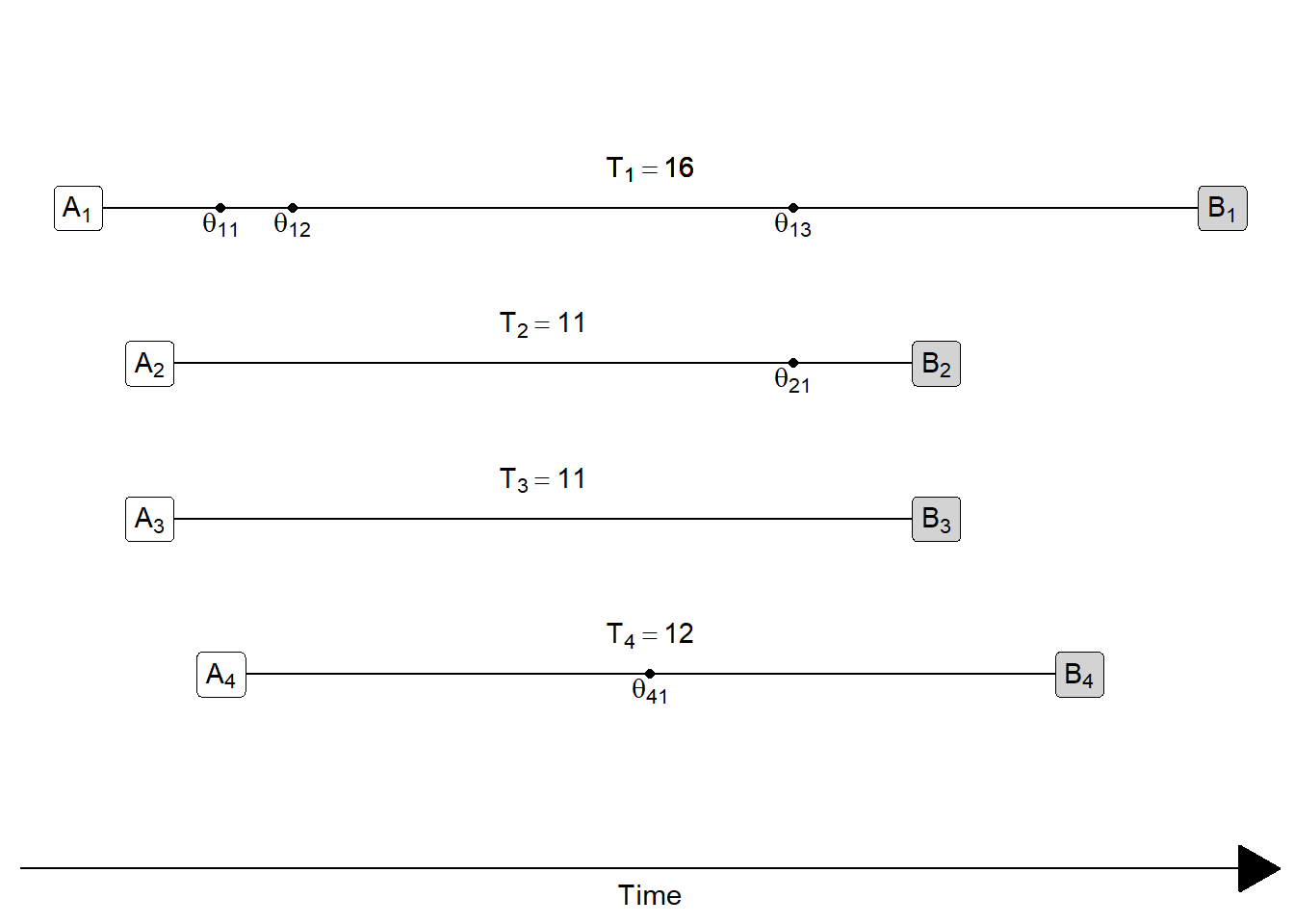
How many occurrences of event \(\theta\) in this picture? Tap for answer

5

How many person-periods? Tap for answer

50

What is the life-time rate? Tap for answer

5 \(\div\) 50 = 10%

KEY CONCEPT

Exposure rates weight individuals in the denominator by the number of person-periods they were exposed to the risk of the event.

1.4 Period rates and person-years (er… person-periods)

Period rate: A rate that limits occurrence and exposure time to those experienced by a population during a specific period of time:

\[ \textsf{Rate}[0,T] = \frac{ \textsf{Number of occurrences between time } 0 \textsf{ and } T } { \textsf{Number of person-periods lived between time } 0 \textsf{ and } T } \]

KEY CONCEPT

People can live fractional (i.e., less than one) person-periods!

Example: By the time you get your final grade for this course on March 23, 2022, you’ll have lived 81 person-days in 2022 so far, which is 22.2% of a person-year…

… unless, of course, you were born this year! 😆

Either way, congrats. 🥂

Let’s illustrate with a toy example:

• A population of 7 people
• Observed over 1 calendar year…

First, let’s look at the lifelines of each individual in the population…

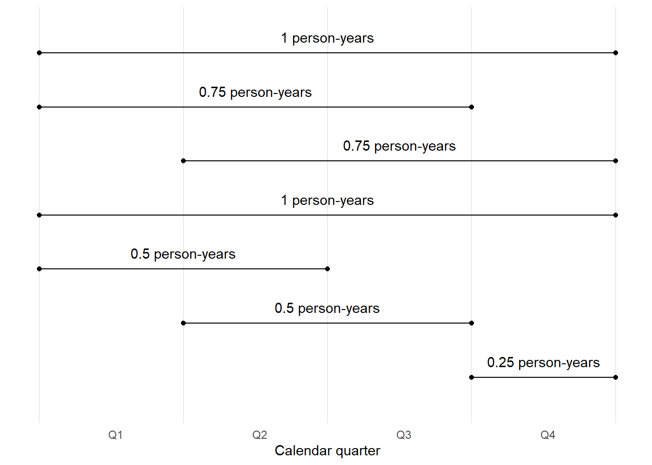
Now, let’s look at how those life lines add up to person-years per quarter…

This shows how the person-years changes from quarter to quarter.

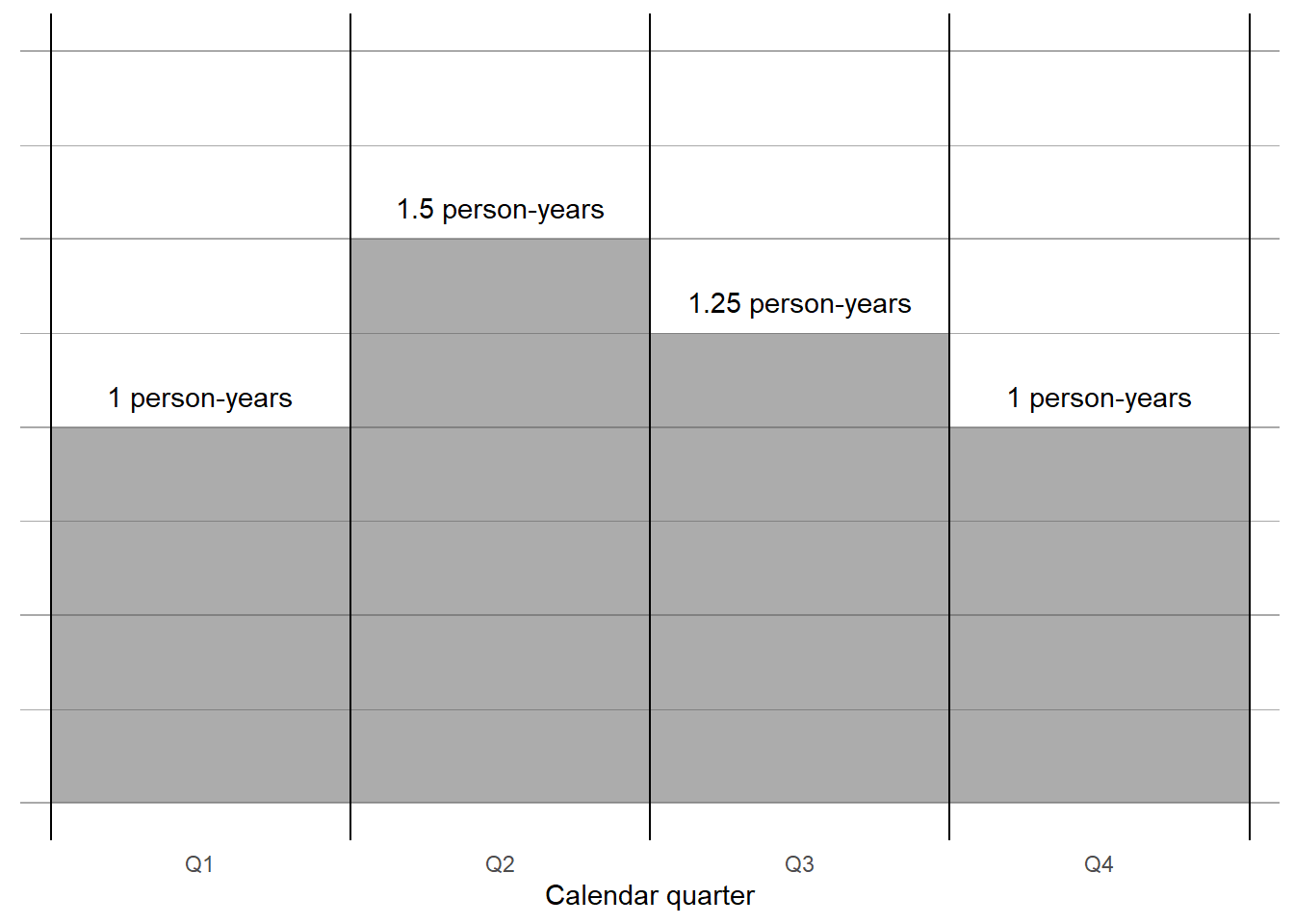
Let’s write down what’s going on:

\(\begin{align} PY[0,1] &= \textsf{(The total person-years lived that year)} \\ &4 \times 0.25 \textsf{ (4 people alive during Q1 times length of quarter in years)} \\ &6 \times 0.25 \textsf{ (6 people were alive in Q2)} \\ &5 \times 0.25 \textsf{ (5 folks in Q3)} \\ &4 \times 0.25 \textsf{ (4 folks in Q4)} \\ &= 19 \times 0.25 \textsf{ (Total number of person-quarters times length of a quarter)} \\ &= 4.75 \text{ (The answer!)} \end{align}\)

Using conventional notation:

\(PY[0,1] = \sum_1^4 N_i \times \Delta_i\)

• \(N_i\): Number of persons alive in the \(i\)^th quarter of the year
• \(\Delta_i\): Fraction of a year represented by that quarter (0.25 if the whole quarter is represented)
  
  

Or more generally, for \(P\) discrete chunks of a period of potentially unequal length:

\(PY[0,T] = \sum_1^{P} N_i \times \Delta_i\)

What would \(\Delta_i\) equal if we counted people each day in 2021? Tap for answer

\(\frac{1}{365}\)

• For 2024, it would be 366 because it’s a leap year
• If our rate spanned across a multiple of four years, it would be 365.25 to account for leap and non-leap years
• Why would \(\Delta_i\) be tedious to calculate if we did monthly counts?

What would \(N_i\) represent if we counted people each day in a year? Tap for answer

Number of persons alive on the \(i\)^th day of the year

How could we express \(PY[0,1]\) mathematically if we were constantly counting people ad nauseum in infinitessimally small units of time of length \(dt\)? Tap for answer

\(PY[0,1] = \int_0^1 N(t) \cdot dt\)

Or for arbitrary period length \(T\): \(PY[0,T] = \int_0^T N(t) \cdot dt\)

🤓 Hypothetically, the most frequent count cadence possible is each chronon, and theoretically the most frequent count cadence possible is the Planck time, so maybe that integral is in the end a continuous approximation of quantized time. 🤓

1.5 Principal period rates in demography

• All of these rates are for an entire population
• For each rate, think about this mangled quote from PHG pg. 7 ¶ 5:

As is especially clear from our definition of the crude rate of in-migration, the connection between exposure and event is not always precise in demography

Crude birth rate:

\[\begin{align} CBR[0,T] &= \frac{\textsf{Number of births between times } 0 \textsf{ and } T} {\textsf{Person-years lived between times } 0 \textsf{ and } T} \\ &= \frac{B[0,T]}{PY[0,T]} \end{align}\]

Crude death rate:

\[\begin{align} CDR[0,T] &= \frac{\textsf{Number of deaths between times } 0 \textsf{ and } T} {\textsf{Person-years lived between times } 0 \textsf{ and } T} \\ &= \frac{D[0,T]}{PY[0,T]} \end{align}\]

Crude rate of in-migration:

\[\begin{align} CRIM[0,T] &= \frac{\textsf{Number of in-migrations between times } 0 \textsf{ and } T} {\textsf{Person-years lived between times } 0 \textsf{ and } T} \\ &= \frac{I[0,T]}{PY[0,T]} \end{align}\]

Crude rate of out-migration:

\[\begin{align} CROM[0,T] &= \frac{\textsf{Number of out-migrations between times } 0 \textsf{ and } T} {\textsf{Person-years lived between times } 0 \textsf{ and } T} \\ &= \frac{O[0,T]}{PY[0,T]} \end{align}\]

CROM!

1.6 Growth rates in demography

Measuring population growth has many uses in traditional demography, such as:

Assessing and mitigating risk of Malthusian traps in resource allocation due to diminishing marginal returns

From CORE econ’s The Economy textbook, Figure 2.15: https://www.core-econ.org/the-economy/book/text/02.html#malthusian-economics-the-effect-of-technological-improvement

Assessing and mitigating risks that slow growth leads to population aging

• What impact does this have on the Social Security system?
• What impact does this have on age patterns of socio-political power?

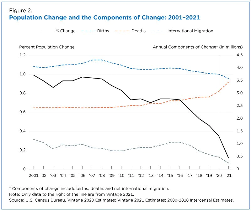
From U.S. Census Bureau: https://www.census.gov/library/stories/2021/12/us-population-grew-in-2021-slowest-rate-since-founding-of-the-nation.html

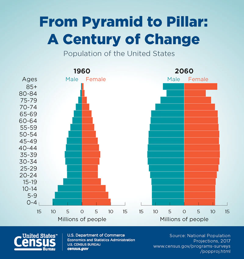
From U.S. Census Bureau: https://www.census.gov/library/visualizations/2018/comm/century-of-change.html

Outside of human demography, tracking how human consumption impacts food stock growth is important and sometimes depressing:

By Food and Agriculture Organization of the United Nations (FAO) - http://www.fao.org/3/ca0191en/ca0191en.pdf, CC BY-SA 3.0 igo, https://commons.wikimedia.org/w/index.php?curid=77504632

DEMOGRAPHY & DATA SCIENCE

Customer demand vs. workforce supply: Challenges to company scale

If high attrition causes employee headcount to grow too slowly relative to demand

• Not enough workers to meet customer demand
• Increased costs to backfill workers who leave
• If your hiring rate is also very high, increased risk of labor market saturation

Even before the pandemic, previously unreported data shows, Amazon lost about 3 percent of its hourly associates each week, meaning the turnover among its work force was roughly 150 percent a year. That rate, almost double that of the retail and logistics industries, has made some executives worry about running out of workers across America.

– Reporting by Jodie Kantor, Karen Weise, and Grace Ashford in the New York Times: https://www.nytimes.com/interactive/2021/06/15/us/amazon-workers.html

1.6.1 Crude growth rate

The crude growth rate combines the Principal period rates in demography into an expression of how a population grows between two time points

Recall the balancing equation:

\[N(T) = N[0] + B[0,T] - D[0,T] + I[0,T] - O[0,T]\]

Using some high school algebra, replace the “?” in the equation below:

\[ \frac{\textsf{?}}{PY[0,T]} = \frac{B[0,T]}{PY[0,T]} - \frac{D[0,T]}{PY[0,T]} + \frac{I[0,T]}{PY[0,T]} - \frac{O[0,T]}{PY[0,T]} \] Tap for answer

\(N(T) - N(0)\) (The period change in population count)

Step 1: Subtract \(N(0)\) from both sides

Step 2: Divide both sides by person-years \(PY[0,T]\)

Putting it all together and substituting in the principal period rates:

\[CGR[0,T] = \frac{N(T) - N(0)}{PY[0,T]} = \textsf{?}\] Tap for answer

\[CBR[0,T] - CDR[0,T] + CRIM[0,T] - CROM[0,T]\]

Arranging by rates related to enters vs. exits Tap for answer

\[\begin{align} CGR[0,T] &= \\ &CBR[0,T] - CDR[0,T] \textsf{ (Crude rate of natural increase } CRNI[0,T] \textsf{)}\\ &+ CRIM[0,T] - CROM[0,T] \textsf{ (Crude rate of net migration } CRNM[0,T] \textsf{)} \end{align}\]

1.6.2 Instantaneous growth rate

CGR measures growth between two time points \(0\) and \(T\), but what about the pace of population growth at a specific point in time \(0 < t < T\)?

• Define period length \(\Delta t\)
• Population change \(N(t + \Delta t) - N(t) = \Delta N(t)\) (Just a generalization of \(N(1) - N(0)\))
• Person-years lived now \(N(t)\Delta t\) (Note similarity to \(PY[0,T] = \sum_1^{P} N_i \times \Delta_i\). Here, \(P = 1\) since we are concerned with only one small interval of time for the whole period.)
• So crude growth rate now \(r(t) = \frac{\Delta N(t)}{N(t) \Delta t}\)

KEY CONCEPT

Instantaneous growth rate is essentially a crude growth rate over tiny period of length \(\Delta t \rightarrow 0\)

Mathematically¹¹:

\[\begin{equation} r(t) = \lim_{\Delta t \to 0} \frac{\Delta N(t)}{N(t) \Delta t} =\frac{d \text{ln}\left[N(t)\right]}{dt} \tag{1.1} \end{equation}\]

We can do algebra and some calculus using Equation (1.1) to express how instantaneous growth accumulates between times \(0\) and \(T\)¹²:

\[\begin{equation} \frac{N(T)}{N(0)} = e^{\int_0^T r(t)dt} \tag{1.2} \end{equation}\]

• Left-hand side: Ratio of ending to starting population size
• Right-hand side: Expression for cumulative growth

Re-arranging:

\[\begin{equation} N(T) = N(0)e^{\int_0^T r(t)dt} \tag{1.3} \end{equation}\]

Assuming constant growth rate \(r^*\) (and sparing derivation on PHG pg. 11):

\[\begin{equation} N(T) = N(0)e^{r^{*} T} \tag{1.4} \end{equation}\]

Dividing both sides by starting population \(N(0)\), we see get an expression for the cumulative growth between times \(0\) and \(T\) under constant rate \(r^*\):

\[\begin{equation} \frac{N(T)}{N(0)} = e^{r^* T} \tag{1.5} \end{equation}\]

Taking the logarithm of both sides of Equation (1.5) and dividing by \(T\) gives us the constant growth rate \(r^*\) between times \(0\) and \(T\):

\[\begin{equation} r^{*} = \frac{\text{ln} \left[\frac{N(T)}{N(0)}\right]}{T} \tag{1.6} \end{equation}\]

1.6.3 Mean annualized growth rate

If we take the logarithm of both sides of (1.2) then divided by \(T\), we get:

\[ \frac{\int_0^T r(t)dt}{T} = \frac{\text{ln} \left[\frac{N(T)}{N(0)}\right]}{T} \]

The left-hand side is just the mean growth rate \(\bar{r}[0,T]\), so:

\[\begin{equation} \bar{r}[0,T] = \frac{\text{ln} \left[\frac{N(T)}{N(0)}\right]}{T} \tag{1.7} \end{equation}\]

The left-hand side is known as the mean annualized growth rate.

1.6.4 Doubling time

If population doubles:

• \(N(T)/N(0) = 2\) (definition of doubling)
• So \(\text{ln}\left[N(T)/N(0)\right] = \text{ln}[2] \approx 0.693\)

Assuming constant growth \(r^*\) and plugging 0.693 into Equation (1.6):

\[\textsf{Doubling time} \approx \frac{0.693}{r^*}\]

1.6.5 Comparison of crude growth rate and mean annualized growth rate

Why does \(CGR = \overline{r}\) only when growth rate is constant? Let’s examine three scenarios: early growth, late growth, and constant growth.

Look at the picture below:

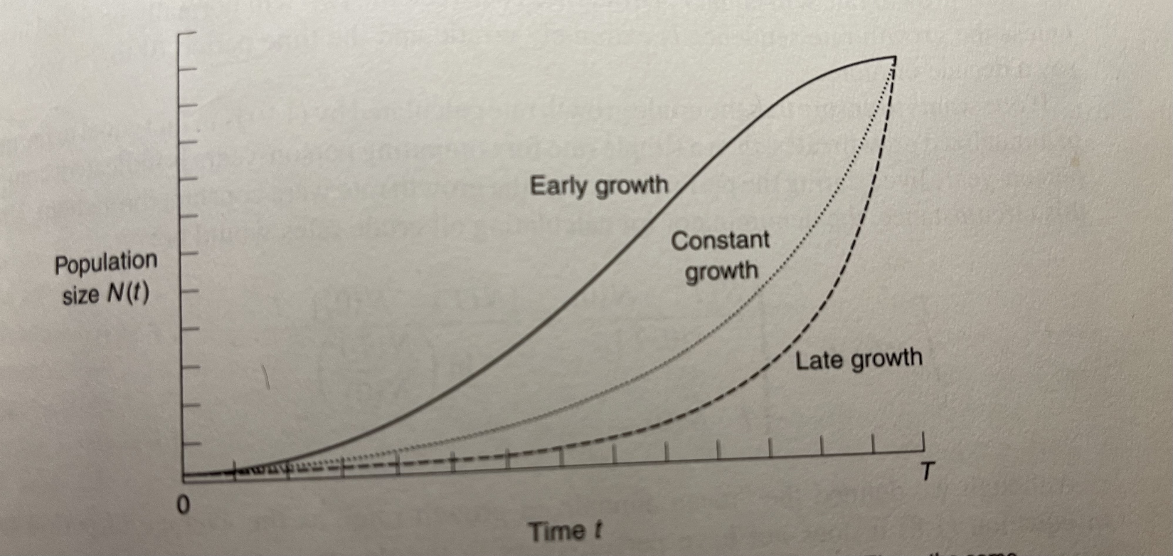
Fig 1.2 from PHG. Three scenarios of within-period growth

• Starting and ending population sizes \(N(0)\) and \(N(T)\) are all the same
• Thus numerators of the crude growth rates \(N(0) - N(T)\) are all the same
• Yet person years (areas under the curves) definitely aren’t the same! That is:

\[PY[0,T]_{\text{early growth}} \neq PY[0,T]_{\text{late growth}} \neq PY[0,T]_{\text{constant growth}}\]

• Therefore the crude growth rates won’t be equal either, that is:

\[ \frac{N(0) - N(T)}{PY[0,T]_{\text{early growth}}} \neq \frac{N(0) - N(T)}{PY[0,T]_{\text{late growth}}} \neq \frac{N(0) - N(T)}{PY[0,T]_{\text{constant growth}}} = r^* \]

• Under constant growth rate \(r^*[0,T]\), person-years lived is:

\[ \require{cancel} PY[0,T]_{\text{constant growth}} = \frac{N(T) - N(0)}{r^*} \]

• Thus CGR under \(r^*[0,1]\) is:

\[ CGR[0,T] = \frac{N(T) - N(0)}{\left[\frac{N(T) - N(0)}{r^*}\right]} = \left[\bcancel{N(T) - N(0)}\right] \cdot \frac{r^*}{\bcancel{N(T) - N(0)}} = r^* \]

• Meanwhile, under \(r^*[0,1]\):

\[ \overline{r}[0,T] = \frac{1}{T}\int_0^Tr^*dt=r^* \]

KEY CONCEPT

With few exceptions, crude growth rate and mean annualized growth rate are not equal unless there is constant growth rate \(r^*\).

Under what circumstances of growth rates and period lengths could we reasonably assume constant growth rate?

If period length is small relative to the pace at which growth rates change

1.7 Estimating period person-periods

• Often, we don’t have access to data on individual lifelines
• Consequence: We have to estimate person-periods to calculate rates

Method 1: Assume constant growth rate \(r\) during the period

We just saw that under constant growth rate \(r^*\):

\[ r^* = CGR[0,T] = \frac{N(T) - N(0)}{PY[0,T]} \]

Solving this equation for \(PY[0,T]\) yields:

\[ PY[0,T] = \frac{N(T) - N(0)}{r^*} \]

Plugging in the right-hand side of Equation (1.6) (our original expression for \(r^*\) before we found it was also equal to \(CGR[0,T]\)) and simplifying yields a handy approximation of person-years that requires only the starting and ending population size and the period length:

\[\begin{equation} PY[0,T] = \frac{ \left[N(T) - N(0)\right] \cdot T }{ \text{ln}\left[\frac{N(T)}{N(0)}\right] } \tag{1.8} \end{equation}\]

If the number of years \(T = 1\), this becomes:

\[ PY[0,1] = \frac{N(1) - N(0)}{ \text{ln}\left[\frac{N(1)}{N(0)}\right] } \]

Method 2: Use mid-period population

• Often, demographers don’t have both start and ending population
• Instead, they have a mid-period population count
• Example: Decennial U.S. Census
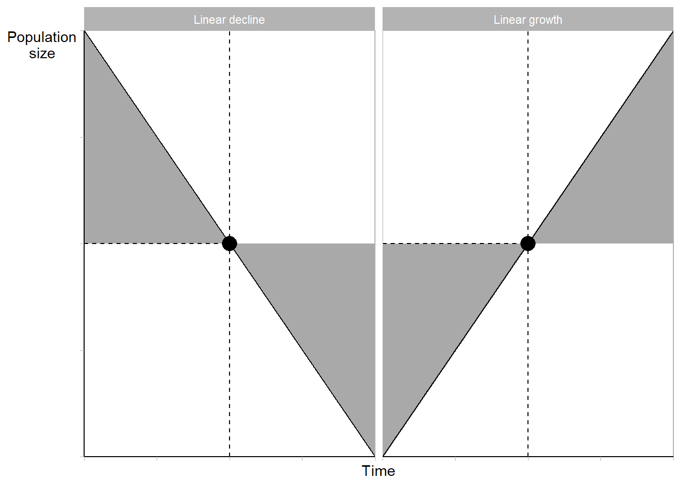
• Mid-period population estimate works best when within-period growth is linear
  

Below are two scenarios of linear population change.

• The black dot shows when within-period population = \(PY[0,1]\)
• Notice how it’s at mid-period
• Note how the mid-period’s under-estimate in one half of the year is balanced by an over-estimate in the other half of the year

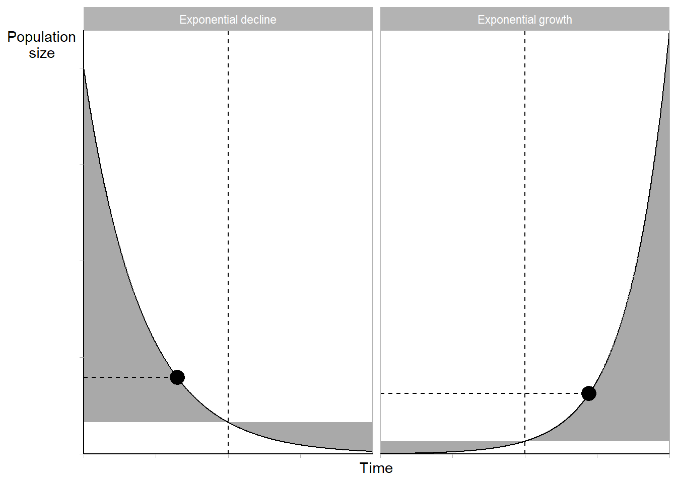
Below are scenarios of exponentially changing populations.

• Notice how mid-period population \(\neq PY[0,1]\)
• Mid-period population under-estimates \(PY[0,1]\) in both cases. Why?

As periods get shorter, the linear approximation gets better

Check it out by zooming in on any point along the population curve below

Method 3: Average of starting and ending population counts

• Sometimes, you don’t have mid-period population \(N(T/2)\)
• So long as you’ve collected data in \(\geq\) 2 consecutive years, you’ve got \(N(0)\) and \(N(T)\)
• Like mid-period population, the average \(\left(N(0) + N(T)\right)/2\) also assumes linear growth

Why does average of starting and ending population assume linear growth? Tap for answer

Remember the midpoint formula for the mid-point between two points on a line?

\[\left(x_m,y_m\right) = \left(\frac{x_1+x_2}{2},\frac{y_1+y_2}{2}\right)\]

Draw a line between \(N(0)\) at time \(0\) and \(N(T)\) at time \(T\).

Plug in for times \(0\) and \(T\) for the \(x_i\) values and populations \(N(t)\) for for \(y_i\)

\[\left(t_m,N_m\right) = \left(\frac{0+T}{2},\frac{N(0)+N(1)}{2}\right) = \left(T/2,\frac{N(0)+N(1)}{2}\right)\]

• Starting-ending average \(\left(N(0)+N(1)\right/2\) is the mid-points’s \(y\) coordinate
• Mid-period \(T/2\) is the mid-point’s \(x\) coordinate
• Therefore the starting-ending average occurs at the mid-period
• Recall that a mid-period approximation assumes linear \(N(t)\)

Since both a mid-period approximation and a start-ending average approximation of \(PY\) assume \(N(T)\) is linear, does that mean they produce the same estimate of \(PY\)?

Not unless \(N(t)\) is in fact linear.

• With mid-period approximation, you assume \(PY = N(T/2) = \frac{1}{2} \left[N(0) + N(T)\right]\) but don’t know \(N(0)\) or \(N(T)\)
• With start-ending average, you assume the same thing, but don’t know \(N(T/2)\)
• Yet if \(N(t)\) is non-linear, \(N(T/2) \neq \frac{1}{2} \left[N(0) + N(T)\right]\)

Method 4: Average of population counts at evenly spaced intervals

• Recall \(PY[0,T] = \sum_{i=1}^{P} N_i \times \Delta_i\)
• For \(P\) equally-sized intervals, this becomes \(PY[0,T] = \sum_1^{P} N_i \times \Delta = \sum_1^{P} N_i \times \frac{1}{P}\)
• This is simply the average of the per-interval population counts
• Higher resolution (i.e., higher \(P\)) means better \(PY[0,T]\) approximation

To illustrate, let’s draw some graphs of average mid-interval estimates at different resolutions.

DEMOGRAPHY & DATA SCIENCE

The promise (and peril) of knowing exact person years

In many business settings, data scientists have access to exact dates when individuals enter and exit a population.

What advantages does this provide? Tap for answer

• Precise estimation of person-periods
• Thus precise estimation of rates
• Flexible aggregation of occurrences in person-periods

Here’s an example of the flexibility of exact person year data. Recall the attrition dataset we worked with in our section on the balancing equation

Below is again a table of the raw data. Which variable would be summed into the numerator of an all-cause termination rate? The denominator? Tap for answer

• Sum of left_company is the occurrence in the numerator
• Sum of tenure is the person-periods (specifically person-months) in the denominator

Below is the sum of terminations (number_terminations) and person-months (employee_months) for every combination of variables gender, age, industry, commute_type, manager_gender, along with the resulting annualized_termination_rate. How is an annual termination rate derived from terminations and person-months?

• If you already have the monthly rate: Multiply it by 12
• Or you could have divided employee_months by 12 to get employee_years

The beauty of exact person-periods is now we can get the same rates for a grouping of variables in one of two ways:

• If starting with individual-level data, sum the individual occurrences and person-periods, then calculate the rate
• If starting with pre-aggregated data, sum the aggregated occurrences and person-periods, then calculate the rate

Below is an example, summing the aggregates above to derive annualized termination rates by gender:

Here is a table created from individual-level data, yielding the same answer:

What types of errors would you expect to see in exact person-year data? Tap for answer

• Exit date happened before entrance date
• Missing exit date even if individual labeled as an exit
• Missing entrance date even if there is an exit date
• Exit and entrance dates both far into the future
• Forgetting far-future exit dates are default values for no event

I have seen all of these and more. Thank now about how you’d deal with them.

1.8 The concept of a cohort

A cohort is an a group of individuals in a population that experience a specific event during a specific time interval.

• Example: People born in the U.S between Jan 1 and Dec 31, 1992

Returning to our lifelines plot:

• Red rectangle shows time interval for qualifying events \(\theta\)

Which individuals are in the cohort? Tap for answer

\(A_4\) only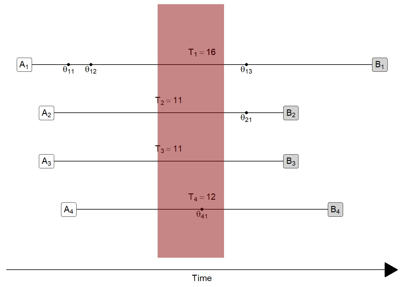

Can you think of any examples of a cohort outside of traditional demography?

• Customer analytics?
• Employee analytics?
• Mechanical engineering?
• Plant biology?
• Something else?

1.9 Probabilities of occurrence of events

KEY CONCEPT

Probabilities measure the chance an event occurs in a cohort within a specific timeframe

\[ \textsf{Probability} = \frac{ \textsf{Number of occurrences } }{ \color{darkorange}{\textsf{Number of preceding events or trials}} } \]

Probabilities also specify a window of observation from…

• when the “preceding event or trial” qualifies for inclusion in the cohort…
• … until either the event occurs or the individual stops being observed

The maximal observation time needs to be same for each member of the cohort

Therefore each individual counted in the denominator needs to have been observed for at least as long as the duration of the observation window

Rates measure the the pace of occurrences per person-year in a population

\[ \textsf{Rate} = \frac{ \textsf{Number of occurrences} }{ \color{dodgerblue}{\textsf{Number of person-periods lived}} } \]

Rates specify a window of observation, as well, but its starting point is not defined by entry of an individual into a cohort.

Instead, it’s defined by the start of the period of observation.

All occurrences and person-periods lived within observation window are counted

No occurrences or person-periods outside the observation window are counted

A lot of this will make way more sense when we study Lexis diagrams

Why does a probability require an observation window with a starting and ending point? Tap for answer

Because if you don’t specify the end of your observation period, somebody or something else will!

Example: All humans eventually die so the following probability is approximately equal to unity (aka 100%) and thus not all that useful:

\[ \frac{ \begin{pmatrix} \textsf{Number of deaths among people born in 1992} \\ \textsf{from now until the heat death of the universe} \end{pmatrix} } {(\textsf{Number of people born in 1992})} \]

In the long run, we are all dead

– John Maynard Keynes